Scratch 'n Win Blues
Alignments to Content Standards:
S-IC.B.4
Task
Many large retail stores and restaurants offer special discounts and free gifts to customers throughout the year. In some cases (particularly fast-food restaurants), some form of “instant win” contest takes place where a customer earns a ticket with a particular food purchase. The ticket states that the customer either has won a food/beverage prize with the ticket (for example, “Instant Win: Free 12 oz. soda!”) or has not won anything with the ticket (for example, “Sorry, you are not a winner. Please play again soon.”)
A certain fast-food restaurant chain offers such a contest in a “scratch ‘n win” format where customers must scratch off a silver coating on a ticket to reveal the outcome. In its commercials, the restaurant chain says that “1 in 5 tickets is a Winner.” However, due to some unfortunate printing and shipping errors, there is now concern that fewer winning tickets have been distributed than originally planned and that the true proportion of winners is in fact less than the 0.20 that was claimed by the “1 in 5 tickets is a Winner” statement. The restaurant chain’s management does not want to get in trouble with the public and be accused of fraud, so they decide to perform some sampling to see if a winning proportion of 0.20 is plausible for the population of tickets that were distributed. They decide to ask the local owners at each of the chain’s 35 most popular locations to conduct some sampling.
Random Sampling
If random sampling is used, it is reasonable for the restaurant management to use the proportion of winning tickets in a given sample (a sample proportion) to estimate the proportion of winning tickets in the entire population (the population proportion). For now, we will assume that the population of tickets is extremely large, that the local owners will use a randomization method to select the customers to approach, and that the customers who are approached about their tickets will answer truthfully.
Management knows that even if the population proportion of winning tickets is actually 0.20 on occasion, the sample proportions will have values that are less than 0.20 due to natural sampling variability. However, they also want to be confident that a population proportion of 0.20 for the winning tickets is plausible.
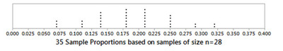
The results of one day of this sampling are shown below. There are 35 observations, and each observation (dot) represents the sample proportion obtained from a given restaurant based on a random sample of 28 tickets at the restaurant. (Each restaurant randomly selected 4 tickets per hour for 7 hours.)
1. None of the sample proportions appear to be exactly equal to 0.20. Explain why obtaining a sample proportion of 0.20 is not possible when using a sample of size 28.
2. According to the dotplot, how many of these 35 sample proportions are below 0.20? Based on these 35 observations, what is the probability that a randomly selected location’s sample proportion was below 0.20?
3. By visual inspection of the dotplot distribution, estimate the values in the 5-number summary for these 35 sample proportions and comment on the shape, center, and range of the distribution.
The important questions for the restaurant chain’s management are: do the results of this day's sampling raise concern about the “1 in 5 tickets is a Winner” claim? Could the actual population proportion of winning tickets actually be less than 0.20?
4. Use the dotplot and/or the analysis you've performed above to address that question. Be thorough and mention any information that would encourage you to dismiss the “1 in 5 tickets is a Winner” claim. Do you feel there is enough evidence to challenge the “1 in 5 tickets is a Winner” claim, or do you feel that the claim should be “left alone” and not disputed?
A Larger Sample Size
Even though the sampling accounted for 980 total tickets (980 = 28 tickets each * 35 locations), some of the company’s executives were concerned that only 28 tickets were sampled at each restaurant. In an urgent memo, management now decides to ask their local owners to now sample 345 tickets in each of the 35 locations (that’s about 49 or 50 tickets per hour for 7 hours). A dotplot showing the sample proportions from the 35 restaurant locations on this second day of sampling (when the sample size of 345 tickets was used at each location) is as follows:

Keep in mind that the population proportion of winning tickets DID NOT CHANGE, only the sample size for each restaurant’s sampling was changed -- specifically it was increased to over 12 times its original size (from 28 tickets to 345 tickets per sample).
Now re-examine the previous questions using this new dotplot.
5. According to this NEW dotplot, how many of these 35 sample proportions are below 0.20?
6. By visual inspection of the dotplot, estimate the values in the 5-number summary for these 35 NEW sample proportions. What is the range of these 35 sample proportions?
7. Using this NEW dotplot, what general information about these 35 sample proportions seems to support the claim that the population proportion of winning tickets is less than 0.20? Do you feel there is enough evidence to challenge the “1 in 5 tickets is a Winner” claim, or do you feel that the claim should be “left alone” and not disputed?
Comparing the Dotplots and the Sample Sizes
8. Which distribution of sample proportions had the smaller range: the distribution based on a sample of size n = 28 or the distribution based samples of size n = 345?
To further examine the effect of sample size, consider the following histograms representing two sampling simulations from the same ticket population. In the first simulation, we imagine that the restaurant management has asked 1000 of its restaurants to randomly sample 28 tickets on a given day. In the second simulation, we imagine that the restaurant management has asked 1000 of its restaurants to randomly sample 345 tickets on given day. Note: both distributions represent the sample proportions from 1000 random samples.


9. Since the local owners who are performing the sampling would pretty much follow whatever instructions they received from restaurant management, would you recommend using a larger sample size or a smaller sample size to estimate the population proportion? Explain.
Margin of Error
In the dotplots given earlier, each dot represented a sample proportion; and each sample proportion is an estimate of the population proportion of winning tickets. When random sampling is used, in the long run, sample proportions generated from many random samples tend to be centered around the actual population proportion. For example, here are the averages of the four distributions shown above:
When the sample was size 28, the average of the 35 sample proportions = 0.189
When the sample was size 345, the average of the 35 sample proportions = 0.169
When the sample was size 28, the average of the 1000 sample proportions = 0.172
When the sample was size 345, the average of the 1000 sample proportions = 0.171
Notice that these four averages are about the same, indicating that the distributions of the sample proportions were all centered at about the same place. Also notice that the “average of all the sample proportions” in all 4 cases was below 0.20; and in 3 of the cases, this average value was quite close to 0.17 -- and that would be a good estimate for the population proportion of winning tickets. Unfortunately, in most analyses, you don’t get to collect many random samples as was done here —you only get to select one random sample for your analysis.
A margin of error is loosely defined as the largest expected size of the difference between an estimate and the actual population value that is being estimated. For example, if you were trying to estimate the population proportion of voters who supported a political candidate and your margin of error was stated as "0.03," that is saying that you would be very confident that the actual population proportion of voters who supported the political candidate is within 0.03 of your sample estimate. In other words, if you obtained a sample proportion of 0.45 and your margin of error was 0.03, you would be very confident that the actual population proportion would be somewhere between 0.42 (that's 0.45 – 0.03) and 0.48 (that's 0.45 + 0.03).
One informal way of developing a margin of error from a simulation is to compute the value that is the range of the simulation’s results divided by 2 (margin of error = range/2). For the first simulation histogram (the one based on samples of size n = 28), this informal margin of error value would be roughly 0.20 (you can confirm this above). If the true population proportion was in fact 0.17, that value would be within the margin of error of nearly every one of the 1000 estimates. In other words, the value "0.17" would be within plus or minus 0.20 of almost any of the 1000 estimates in the histogram. (In fact, “0.17” is within plus or minus 0.20 of 997 of the 1000 estimates.)
10. If we perform this same informal method of developing a margin of error using the second simulation histogram (the one based on samples of size n = 345), what would the value for the margin of error be approximately? Using this margin of error value, how many of the estimates in the dotplot from Questions 5 – 7 are within this margin of error of the hypothesized population proportion value of 0.20?
11. Generally speaking, do you think that when proper random sampling occurs, the margin of error for estimating a population proportion gets smaller or larger as the sample size increases?
IM Commentary
Although margin of error can be computed by formula, this task is intended to engage students in considering how it can be estimated from examining the results of repeated simple random sampling. This approach should also assist students in developing a more visual sense of what “margin of error” means in terms of estimation.
A key point for students to address up front is that even perfect simple random sampling will not always yield a sample estimate that is equal to the value of the population parameter it is estimating. There will always be some sampling variability. However, students should also realize that using larger samples (properly collected) leads to less sampling variability and thus a smaller margin of error when estimating the population parameter.
Solution
1. 20% of 28 = 5.6; it is not possible to have exactly 5.6 winning tickets as “number of winning tickets” must be an integer.
2. 19 of the 35 sample proportions are below 0.20 (19/35 = 0.5429 or 54.29%). Nearly half of the proportions (0.4571 or 45.71%) are above 0.20 as well. The probability that a randomly selected location’s proportion is less than 0.20 is 0.5429.
3. Actual values:
Minimum Q1 Median Q3 Maximum
.0714 .1429 .1786 .25 .3214
Center: around 0.18 – 0.20 (Midrange = 0.1964)
Shape: nearly symmetric, with most of the observations around 0.20
Range: 0.25
Note: Student's answers should be close to these values but may not be quite this precise since the actual data values are not presented. However, given the discrete nature of these data, students may figure out from the dotplot that the minimum value of 0.0714 represents 2 successes out of 28, the Q1 represents 4 out of 28, and so on.
4. Concern: Slightly over half of the sample proportion values were below 0.20. However, with many of the values near 0.20, nearly half of the values above 0.20, and the center near 0.20, it would be difficult to challenge the claim that the population proportion of winning tickets is 0.20.
5. 34 of the 35 sample proportions are below 0.20.
6. Actual values:
Minimum Q1 Median Q3 Maximum
.1391 .1594 .1652 .1826 .2145
Range: less than 0.08 (.0754)
7. Since 34 of the 35 sample proportions are less than 0.20, there is now some stronger evidence that the population proportion of winning tickets might be less than 0.20. However, because there is variability in all sampling, we have not proven that the population proportion is less than 0.20.
8. Using samples of size 345 resulted in a distribution with a smaller range. The sample proportions didn’t vary as widely.
9. The larger sample sizes are yielding estimates that do not vary as much. The larger sample size is preferable.
10. It is roughly 0.06 (.0594) It appears that 33 of the 35 sample proportions could say that 0.20 is within this margin of error.
11. Generally, the margin of error would decrease as sample size increases.
Scratch 'n Win Blues
Many large retail stores and restaurants offer special discounts and free gifts to customers throughout the year. In some cases (particularly fast-food restaurants), some form of “instant win” contest takes place where a customer earns a ticket with a particular food purchase. The ticket states that the customer either has won a food/beverage prize with the ticket (for example, “Instant Win: Free 12 oz. soda!”) or has not won anything with the ticket (for example, “Sorry, you are not a winner. Please play again soon.”)
A certain fast-food restaurant chain offers such a contest in a “scratch ‘n win” format where customers must scratch off a silver coating on a ticket to reveal the outcome. In its commercials, the restaurant chain says that “1 in 5 tickets is a Winner.” However, due to some unfortunate printing and shipping errors, there is now concern that fewer winning tickets have been distributed than originally planned and that the true proportion of winners is in fact less than the 0.20 that was claimed by the “1 in 5 tickets is a Winner” statement. The restaurant chain’s management does not want to get in trouble with the public and be accused of fraud, so they decide to perform some sampling to see if a winning proportion of 0.20 is plausible for the population of tickets that were distributed. They decide to ask the local owners at each of the chain’s 35 most popular locations to conduct some sampling.
Random Sampling
If random sampling is used, it is reasonable for the restaurant management to use the proportion of winning tickets in a given sample (a sample proportion) to estimate the proportion of winning tickets in the entire population (the population proportion). For now, we will assume that the population of tickets is extremely large, that the local owners will use a randomization method to select the customers to approach, and that the customers who are approached about their tickets will answer truthfully.
Management knows that even if the population proportion of winning tickets is actually 0.20 on occasion, the sample proportions will have values that are less than 0.20 due to natural sampling variability. However, they also want to be confident that a population proportion of 0.20 for the winning tickets is plausible.
The results of one day of this sampling are shown below. There are 35 observations, and each observation (dot) represents the sample proportion obtained from a given restaurant based on a random sample of 28 tickets at the restaurant. (Each restaurant randomly selected 4 tickets per hour for 7 hours.)
1. None of the sample proportions appear to be exactly equal to 0.20. Explain why obtaining a sample proportion of 0.20 is not possible when using a sample of size 28.
2. According to the dotplot, how many of these 35 sample proportions are below 0.20? Based on these 35 observations, what is the probability that a randomly selected location’s sample proportion was below 0.20?
3. By visual inspection of the dotplot distribution, estimate the values in the 5-number summary for these 35 sample proportions and comment on the shape, center, and range of the distribution.
The important questions for the restaurant chain’s management are: do the results of this day's sampling raise concern about the “1 in 5 tickets is a Winner” claim? Could the actual population proportion of winning tickets actually be less than 0.20?
4. Use the dotplot and/or the analysis you've performed above to address that question. Be thorough and mention any information that would encourage you to dismiss the “1 in 5 tickets is a Winner” claim. Do you feel there is enough evidence to challenge the “1 in 5 tickets is a Winner” claim, or do you feel that the claim should be “left alone” and not disputed?
A Larger Sample Size
Even though the sampling accounted for 980 total tickets (980 = 28 tickets each * 35 locations), some of the company’s executives were concerned that only 28 tickets were sampled at each restaurant. In an urgent memo, management now decides to ask their local owners to now sample 345 tickets in each of the 35 locations (that’s about 49 or 50 tickets per hour for 7 hours). A dotplot showing the sample proportions from the 35 restaurant locations on this second day of sampling (when the sample size of 345 tickets was used at each location) is as follows:
Keep in mind that the population proportion of winning tickets DID NOT CHANGE, only the sample size for each restaurant’s sampling was changed -- specifically it was increased to over 12 times its original size (from 28 tickets to 345 tickets per sample).
Now re-examine the previous questions using this new dotplot.
5. According to this NEW dotplot, how many of these 35 sample proportions are below 0.20?
6. By visual inspection of the dotplot, estimate the values in the 5-number summary for these 35 NEW sample proportions. What is the range of these 35 sample proportions?
7. Using this NEW dotplot, what general information about these 35 sample proportions seems to support the claim that the population proportion of winning tickets is less than 0.20? Do you feel there is enough evidence to challenge the “1 in 5 tickets is a Winner” claim, or do you feel that the claim should be “left alone” and not disputed?
Comparing the Dotplots and the Sample Sizes
8. Which distribution of sample proportions had the smaller range: the distribution based on a sample of size n = 28 or the distribution based samples of size n = 345?
To further examine the effect of sample size, consider the following histograms representing two sampling simulations from the same ticket population. In the first simulation, we imagine that the restaurant management has asked 1000 of its restaurants to randomly sample 28 tickets on a given day. In the second simulation, we imagine that the restaurant management has asked 1000 of its restaurants to randomly sample 345 tickets on given day. Note: both distributions represent the sample proportions from 1000 random samples.
9. Since the local owners who are performing the sampling would pretty much follow whatever instructions they received from restaurant management, would you recommend using a larger sample size or a smaller sample size to estimate the population proportion? Explain.
Margin of Error
In the dotplots given earlier, each dot represented a sample proportion; and each sample proportion is an estimate of the population proportion of winning tickets. When random sampling is used, in the long run, sample proportions generated from many random samples tend to be centered around the actual population proportion. For example, here are the averages of the four distributions shown above:
When the sample was size 28, the average of the 35 sample proportions = 0.189
When the sample was size 345, the average of the 35 sample proportions = 0.169
When the sample was size 28, the average of the 1000 sample proportions = 0.172
When the sample was size 345, the average of the 1000 sample proportions = 0.171
Notice that these four averages are about the same, indicating that the distributions of the sample proportions were all centered at about the same place. Also notice that the “average of all the sample proportions” in all 4 cases was below 0.20; and in 3 of the cases, this average value was quite close to 0.17 -- and that would be a good estimate for the population proportion of winning tickets. Unfortunately, in most analyses, you don’t get to collect many random samples as was done here —you only get to select one random sample for your analysis.
A margin of error is loosely defined as the largest expected size of the difference between an estimate and the actual population value that is being estimated. For example, if you were trying to estimate the population proportion of voters who supported a political candidate and your margin of error was stated as "0.03," that is saying that you would be very confident that the actual population proportion of voters who supported the political candidate is within 0.03 of your sample estimate. In other words, if you obtained a sample proportion of 0.45 and your margin of error was 0.03, you would be very confident that the actual population proportion would be somewhere between 0.42 (that's 0.45 – 0.03) and 0.48 (that's 0.45 + 0.03).
One informal way of developing a margin of error from a simulation is to compute the value that is the range of the simulation’s results divided by 2 (margin of error = range/2). For the first simulation histogram (the one based on samples of size n = 28), this informal margin of error value would be roughly 0.20 (you can confirm this above). If the true population proportion was in fact 0.17, that value would be within the margin of error of nearly every one of the 1000 estimates. In other words, the value "0.17" would be within plus or minus 0.20 of almost any of the 1000 estimates in the histogram. (In fact, “0.17” is within plus or minus 0.20 of 997 of the 1000 estimates.)
10. If we perform this same informal method of developing a margin of error using the second simulation histogram (the one based on samples of size n = 345), what would the value for the margin of error be approximately? Using this margin of error value, how many of the estimates in the dotplot from Questions 5 – 7 are within this margin of error of the hypothesized population proportion value of 0.20?
11. Generally speaking, do you think that when proper random sampling occurs, the margin of error for estimating a population proportion gets smaller or larger as the sample size increases?